Wrangling Financial Returns with Pandas

Data

The data we wish to investigate are related to three stocks quoted in the NASDAQ 100 index, namely Apple, Google and Facebook, observed in the period Jan-Sept 2020. They are stored in three different .csv files, which can be read and stored using the pandas .read_csv() function into aapl_df, googl_df, and fb_df, respectively.

Each of them contains different trading information on the corresponding stocks, identified by the column Symbol, such as their trading date, represented by Date, the highest and lowest price observed in that trading session, represented by the column High and Low respectively, the opening and closing price, represented by Open and Close, and finally their observed Volume in each session.

A simple inspection of the first five rows of the aapl_df dataframe gives us a better idea of the data we are dealing with:

	Date	High	Low	Open	Volume	Close	Symbol
0	2020-01-02	75.150002	73.797501	74.059998	135480400.0	74.573036	AAPL
1	2020-01-03	75.144997	74.125000	74.287498	146322800.0	73.848030	AAPL
2	2020-01-06	74.989998	73.187500	73.447502	118387200.0	74.436470	AAPL
3	2020-01-07	75.224998	74.370003	74.959999	108872000.0	74.086395	AAPL
4	2020-01-08	76.110001	74.290001	74.290001	132079200.0	75.278160	AAPL

To get a general overview of the dataset under investigation, we can apply the .info() method on the dataset:

aapl_df.info()

<class 'pandas.core.frame.DataFrame'>
RangeIndex: 189 entries, 0 to 188
Data columns (total 7 columns):
 #   Column  Non-Null Count  Dtype  
---  ------  --------------  -----  
 0   Date    189 non-null    object
 1   High    189 non-null    float64
 2   Low     189 non-null    float64
 3   Open    189 non-null    float64
 4   Volume  189 non-null    float64
 5   Close   189 non-null    float64
 6   Symbol  189 non-null    object
dtypes: float64(5), object(2)
memory usage: 10.5+ KB

This gives us a few useful information: from the columns’ type to the shape of the dataset, so that one can easily understand the data at a glance. Note also the information related to the memory used by the pandas.dataFrame object.

Data wrangling

We concatenate the three pandas.DataFrame objects into a single variable, and call it df_all. That will be of type pandas.DataFrame, since we are just concatenating objects belonging to the same class. Note that by default, the pd.concat() function concatenates the dataframe objects by row.

df_all = pd.concat([aapl_df, googl_df, fb_df])
df_all.reset_index(drop=True, inplace=True)

Note that we both reset and drop the original indexes, since rows must be uniquely determined - otherwise, index one will be repeated thrice in df_all.

The dataset stored in df_all is a tidy dataset. We now want to perform aggregating operations with respect to the Close price column, say creating a new pandas.DataFrame object containing as index the Date and as columns the Stock.

This is easily performed by applying the pivot() method on the df_all, which requires three arguments:

• index: the column we wish to have as index of the new dataframe - in this case Date;
  
• columns: the column we wish to have as columns of the new dataframe - in this case Symbol;
  
• values: the column we wish to have as values of the new dataframe - in this case Close.
  

The resulting dataframe is stored into the object pivot_close. At the end, we sort the index using the sort_index() method so that we are sure the index is correctly ordered in ascending order.

pivot_close = df_all.pivot(
    index='Date',
    columns='Symbol',
    values='Close'
).sort_index()

The first five rows of the resulting pivot_close dataframe is shown below:

Symbol	AAPL	FB	GOOGL
Date
2020-01-02	74.573036	209.779999	1368.680054
2020-01-03	73.848030	208.669998	1361.520020
2020-01-06	74.436470	212.600006	1397.810059
2020-01-07	74.086395	213.059998	1395.109985
2020-01-08	75.278160	215.220001	1405.040039

Now the dataset is more compact, since each row represent a trading day, and columns represents the stocks under investigation.

Data Manipulation

As an investor, we would like to know whether we are making money out of our investment. Indeed, at the end of the day, we are happy to know the performance of the stocks in our portfolio. We have different strategies: we might want to compute, for instance, the absolute daily change in the stock value. This is an elementary strategy, but it is efficient to understand the trend.

To compute the difference in price with a time-window of one period (i.e. a day), pandas provides a very interesting method called diff(): this basically computes the absolute difference in price with respect to a time-window of size given by the argument periods, which is by default set to be one. The following function is just a wrapper of the diff() function.

def getting_diff_price(df):
    return df.diff()

absolute_diff_price_df = getting_diff_price(pivot_close)

Symbol	AAPL	FB	GOOGL
Date
2020-01-02	NaN	NaN	NaN
2020-01-03	-0.725006	-1.110001	-7.160034
2020-01-06	0.588440	3.930008	36.290039
2020-01-07	-0.350075	0.459991	-2.700073
2020-01-08	1.191765	2.160004	9.930054

Sometimes, however, that information is useless. Given a book value of the investment, we would like to know whether we are making money with respect to the initial investment. The next function computes the difference between the book value and the current value of the investment - in our case, the single stock.

def getting_diff_price(df):
    return df.apply(lambda x: x-x[0], axis=0)

Since we want to make our life easier, we create a method that ingests two arguments:

• date: the date we wish to measure the performance of our investment;
• data: the dataset of closing prices.

This method is provided below here:

def get_value_investment_at_date(date, data):
    df = data.loc[date].to_frame().T
    df.columns.name = None
    return df

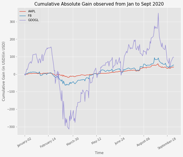
We call both methods in the next snippet; the results is pretty straightforward: in the given date, the stocks’ prices are all above the initial investment.

diff_from_start = getting_diff_price(pivot_close)
get_value_investment_at_date(date='2020-09-30', data=diff_from_start)

	AAPL	FB	GOOGL
2020-09-30	41.236961	52.119995	96.919922

The next figure describes the evolution of the investment results, given in the above dataframe diff_from_start, into a graphical dimension.

Simple Financial Returns to the Rescue!

Can you spot a potential problem in the previous result? Well, one stock - i.e. GOOGL - is expressed in thousands, whereas the others in hundreds.

Typically, a financial investor is more interested in looking at the financial returns rather than computing the absolute difference in price. Let \(P_{t}\) be the price of the security at time t. The simple return between times \(t\) and \(t−1\) is defined as

\[R_t = \frac{P_t}{P_{t-1}}-1\]

In pandas, financial returns can be easily computed by employing the function pct_change(), which basically computes the simple returns as described mathematically above. The following wrapper basically applies this function on each row:

def daily_change(row):
    return row.pct_change()

The following object, called daily_returns, contains the simple financial returns for the three stocks.

daily_returns = pivot_close.apply(lambda x: daily_change(x))

	AAPL	FB	GOOGL
Date
2020-01-02	NaN	NaN	NaN
2020-01-03	-0.009722	-0.005291	-0.005231
2020-01-06	0.007968	0.018834	0.026654
2020-01-07	-0.004703	0.002164	-0.001932
2020-01-08	0.016086	0.010138	0.007118

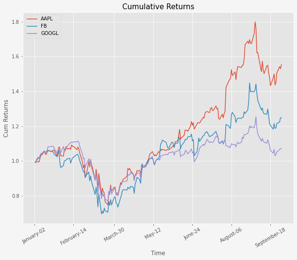
It looks like we have normalized the data, so that each stocks can be easily compared with another one, no matters whether it is expressed in thousands, or any other unit. Since we introduced the simple returns to better understand the investment returns, we now compute the cumulative returns, which basically mimick the logic behind the cumulative difference in price we computed in the previous section. With the only difference that the baseline is now the simple return (instead of the absolute difference in price with respect to the book value price of the investment).

def daily_cum_returns(row):
    return (row + 1).cumprod()

cum_daily_returns = daily_returns.apply(lambda x: daily_cum_returns(x))

The next figure shows the cumulative returns for AAPL, FB and GGOGL.

We now clearly see that AAPL was the stock who surged the most, confirming that simple (but even log) returns should be the starting point of any financial analyst before a deeper investigation.

Conclusions

In this post, we have understood how to employ pandas to perform exploratory financial data analysis. We have understood:

• how to manipulate a financial dataset;
• how to compute absolute difference in price;
• how to compute log returns, and the corresponding cumulative returns.

I hope you have enjoyed it. If you are interested in replicating the results shown here, you can find here the source code of this post. See you in the next post!

Datasets:

• Apple Stock (Jan-Sept 2020)
• Facebook Stock (Jan-Sept 2020)
• Google Stock (Jan-Sept 2020)